Introduction to MLOps: The DevOps of Machine Learning

Every few months, a data scientist on the team shares a Jupyter notebook in Slack, says "the model works, can you deploy it?", and walks away. And every time, the same problems appear. The notebook only runs on their laptop. There's a model.pkl file that nobody can find. Half of the imports are missing from the requirements file. And when it finally runs in production, it quietly starts giving worse answers three weeks later, and nobody notices until a customer complains.

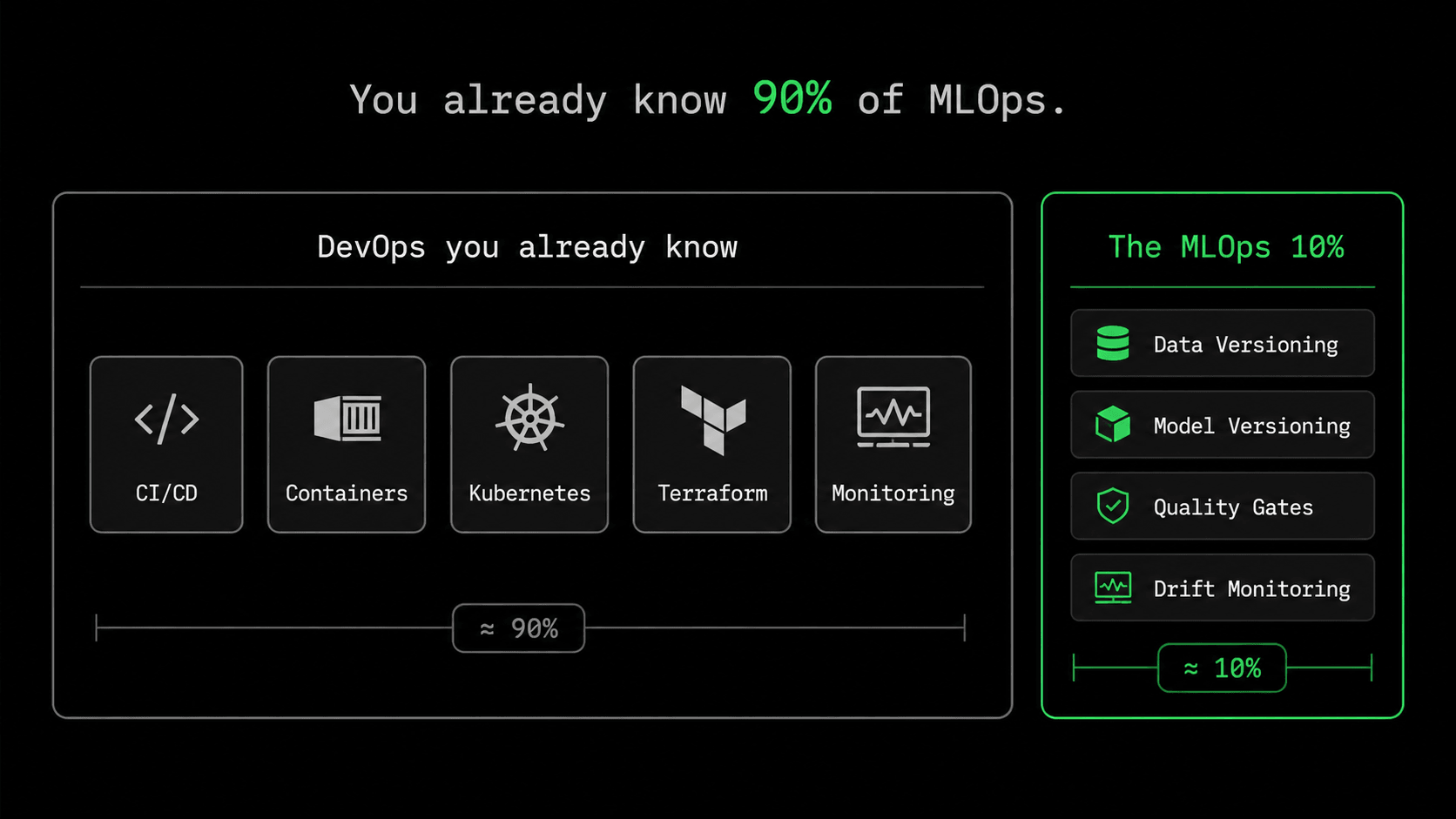
If you're a DevOps or backend engineer, this is how you get pulled into MLOps — whether you planned for it or not. The good news: you already know most of it. CI/CD, containers, Kubernetes, Terraform, monitoring — that covers 90% of the job. This series is about the other 10%: the parts that really are different when you ship a model instead of a web app.

This is the first article in an 11-part series. We'll take one small model and carry it, step by step, to a production setup on AWS — FastAPI, Docker, GitHub Actions, MLflow, DVC data versioning, Kubernetes, Terraform, Prometheus, Grafana, and drift detection. No PhD required. I approach this the same way you would: as the engineer who has to keep the system running at 3am, not as a researcher tuning hyperparameters.

What is MLOps, really?

MLOps is the set of practices for taking a machine learning model from "it works on my laptop" to "it's running reliably in production and someone knows when it breaks." That's it. If you swap "machine learning model" for "web service," you've just described DevOps.

So why does it get its own name and its own tools? Because a model isn't code in the way a REST endpoint is code. A model is three things combined: code, the data it learned from, and a training process that turned that data into numbers. When any one of those three changes, the model's behavior changes, and two of them (the data and the training) live outside of what your Git repo normally tracks.

The mental model I use is simple. In a normal app, the same input always gives the same output until you change the code. With a model, the code can stay untouched for six months and the quality still drops. Why? Because the real world slowly moved away from the data the model was trained on. The code didn't change. The world did. That's the whole problem.

Think of a trained model as a photo of the world, taken at the exact moment of training. The photo never changes. But the world keeps moving. The model learned 2019's prices, and 2019 isn't coming back. The gap between that frozen photo and today is what we call drift, and a big part of this series is about catching that gap before your users do. Drift comes in two forms, which we'll separate later: either the incoming data changes shape (your users moved to mobile), or the rules themselves change (what counted as fraud last quarter isn't what counts this quarter).

The ML lifecycle, from a DevOps lens

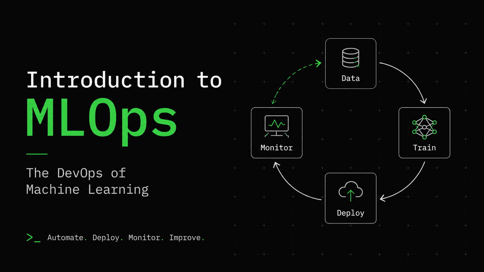
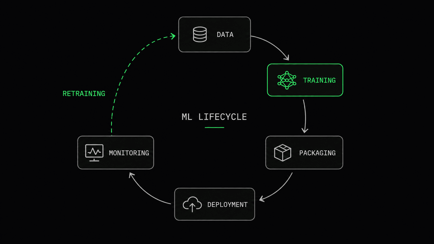
You already know the app lifecycle: write code, test, build, deploy, monitor, repeat. The ML lifecycle is the same loop with two extra stages added at the front and one important feedback arrow at the end.

• →Data — you collect and clean the data the model learns from. Think of this as the source code you didn't write by hand.
• →Training — an offline job turns that data into a model artifact. This is your build, except it can take hours and, unless you pin the random seed, produce a different model each run.
• →Packaging — you wrap the artifact in an API and a container. This part is 100% normal DevOps.
• →Deployment — ship it to Kubernetes / ECS / wherever. Also normal DevOps.
• →Monitoring — watch latency and errors like always, and also watch whether the predictions are still any good.
• →Retraining — when quality drops, you go back to step one with fresh data. This arrow is what makes it a cycle instead of a line.

Notice that four of those six stages are things you already do every day. The two new ones — training and retraining — plus the extra layer of monitoring are what this whole series is about.

Training vs inference: the split everything else hangs off

If you take one idea away from this article, make it this one. Almost every design decision in MLOps comes back to keeping these two things separate.

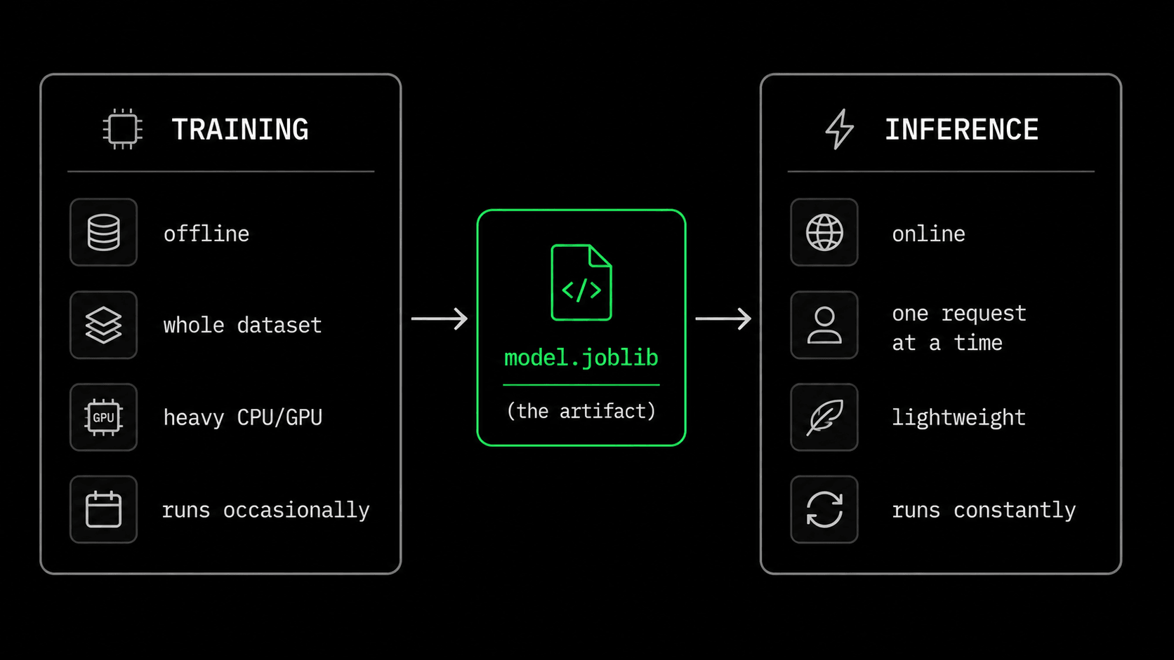
Training is the expensive, offline, occasional job that reads a pile of data and produces a model. It needs lots of CPU or GPU, it needs the whole dataset, and it runs maybe once a day, once a week, or once when someone clicks a button. If it fails, no user notices.

Inference is the cheap, online job that runs all the time: it takes one request and returns one answer. It needs the finished model, but not only the model. A .joblib file isn't self-contained: to load it, you still need scikit-learn installed, ideally the exact version you trained with. Load a model saved with sklearn 1.3 into a 1.5 runtime and you get a version warning at best, or silently wrong predictions at worst. So the inference image pins the sklearn version, but drops the dataset, pandas, and the training code. Inference runs thousands of times a minute, and if it goes down, users notice immediately.

Mixing these two up is the number one beginner mistake. Your production API should never import the training code, never re-read the dataset on startup, and never call .fit() anywhere near a live request. The training job has exactly one job: to hand over a single file — the model artifact.

If you've ever written a multi-stage Dockerfile, you already know this pattern. Training is the builder stage: it pulls in the whole dataset, the heavy libraries, and the GPU toolchain. Inference is the final stage: it copies out one file with COPY --from=builder and throws everything else away. The model artifact is the only thing that crosses that line. Importing training code into your API is the same mistake as shipping gcc and your test fixtures in a production image.

The model artifact: your new deployable

In web development, you deploy a container image. In ML, you deploy the model artifact — a file that stores the trained model. For scikit-learn it's usually a .joblib or .pkl file; for other frameworks it's a .pt, an .onnx, or a folder of weights. Think of it like a .jar you copy into an image, not the image itself: it's passive data. It still needs predict.py, Python, and a pinned sklearn version around it before it can answer anything.

Treat this file the way you treat any build artifact: immutable, versioned, reproducible. And "reproducible" has a catch worth spelling out — notice the random_state=42 in train.py. Without a fixed seed, two runs on the same data grow different trees, and "reproducible" quietly stops being true. Pin the code, the data snapshot, the config, and the seed, and you get the same model every time — just like a build is only reproducible when you also pin your dependencies. Once that holds, debugging a bad prediction becomes one simple question: which artifact was live, and what trained it?

For now, we'll simply keep the artifact next to our code. That's fine for article one. By article five it moves into a Model Registry in MLflow — think of ECR, but for models. Instead of pushing image:sha and promoting it from staging to production, you register model v1, v2, v3 and move the "production" pointer to whichever version earned it. "Which model is live?" becomes a simple lookup, not a guessing game over SSH. (Git LFS looks like a tempting shortcut, but it only versions the bytes, not the data that produced them. That's exactly why a registry is worth having.)

Why DevOps alone isn't enough

You could take a model, wrap it in FastAPI, containerize it, and ship it with the CI/CD pipeline you already have. Honestly, that gets you surprisingly far. So where does plain DevOps stop being enough?

• →Your artifact doesn't fit in Git. Ours is a ~47MB RandomForest, and every retrain would add another 47MB blob to history — a blob Git can never diff or clean up. This is the same wall that pushes people toward Git LFS. You need artifact and data versioning that Git was never built for. (Also: only load a .pkl file you created yourself — unpickling runs arbitrary code.)
• →Passing the tests isn't enough. A unit test asks "is the code correct?". A quality gate asks "is this model better than the one already in production?". That's champion vs challenger: the live model is the champion, your new candidate is the challenger, and CI promotes the challenger only if it beats the champion on a test metric. It's the same shape as a benchmark job that fails a build when p99 latency gets worse. A green build with a worse model really does happen.
• →A model gets worse without any code change. Data drift and concept drift mean a frozen model slowly loses accuracy on its own. Nothing in classic DevOps watches for that, because normal services don't behave this way.
• →Reproducing a deployment needs three things, not one. You need the code version, the data version, and the training config. If you miss any one of them, you can't rebuild the same model.

So MLOps doesn't replace DevOps. It's DevOps plus artifact and data versioning, plus quality gates, plus drift monitoring, plus retraining. Everything we build in this series is a familiar tool doing one of those extra jobs.

Hands-on: train an artifact, then run inference

Let's make that split concrete with about 30 lines of Python. We'll use scikit-learn's California housing dataset to predict median house prices. It's a simple, well-understood regression problem, and that's exactly what we want. The model isn't the point. The workflow is the point.

Start with a clean folder and a virtual environment. This same repo grows across all 10 articles, so start it right.

mkdir mlops && cd mlops
python3 -m venv .venv
source .venv/bin/activate

pip install scikit-learn joblib pandas

Here's train.py. Read the comments — the whole file exists to produce one artifact and then get out of the way.

# train.py — turns data into a model artifact. Runs offline.
import json
from datetime import datetime, timezone
from pathlib import Path

import joblib
from sklearn.datasets import fetch_california_housing
from sklearn.ensemble import RandomForestRegressor
from sklearn.metrics import mean_absolute_error, r2_score
from sklearn.model_selection import train_test_split

MODEL_DIR = Path("model")
FEATURES = ["MedInc", "HouseAge", "AveRooms", "AveBedrms",
            "Population", "AveOccup", "Latitude", "Longitude"]

data = fetch_california_housing()
X_train, X_test, y_train, y_test = train_test_split(
    data.data, data.target, test_size=0.2, random_state=42)

model = RandomForestRegressor(n_estimators=200, max_depth=12, random_state=42)
model.fit(X_train, y_train)

preds = model.predict(X_test)
mae = mean_absolute_error(y_test, preds)
r2 = r2_score(y_test, preds)
print(f"MAE: {mae:.3f}  R2: {r2:.3f}")

MODEL_DIR.mkdir(exist_ok=True)
joblib.dump(model, MODEL_DIR / "model.joblib")

metadata = {
    "model_name": "california-house-price",
    "model_version": "1.0.0",
    "features": FEATURES,
    "metrics": {"mae": round(mae, 4), "r2": round(r2, 4)},
    "trained_at": datetime.now(timezone.utc).isoformat(),
}
(MODEL_DIR / "metadata.json").write_text(json.dumps(metadata, indent=2))
print("Saved model/model.joblib")

Run python train.py. On my machine it printed MAE: 0.346 and R2: 0.792. An MAE of 0.346 means the model is off by about $34,600 on average (the target is in units of $100,000), and an R2 of 0.79 means it explains most of the variation in prices. Good enough. But look at what actually landed on disk — that's the important part.

model/
├── model.joblib      # the artifact — this is what we deploy
└── metadata.json     # what it is, how good it is, when it was made

The metadata.json file records where the artifact came from — the same job a MANIFEST does for a .jar. It travels with the artifact and describes what it is: the model name and version, the exact feature order, the metrics it scored, and when it was trained. When a prediction looks wrong at 3am, those fields answer "what exactly is running, and can I rebuild it?" without opening a notebook.

Now the other half. Notice what predict.py doesn't do: it never imports the training code, never touches the dataset, never calls .fit(). It loads a finished file and asks it a question. This is the code that becomes our production API in the next article.

# predict.py — loads the artifact and runs one prediction. Online.
import json
from pathlib import Path
import joblib

model = joblib.load(Path("model") / "model.joblib")
metadata = json.loads((Path("model") / "metadata.json").read_text())

# One California block group, features in the trained order.
sample = [8.3252, 41.0, 6.9841, 1.0238, 322.0, 2.5556, 37.88, -122.23]

prediction = model.predict([sample])[0]
print(f"Model: {metadata['model_name']} v{metadata['model_version']}")
print(f"Predicted median house value: ${prediction * 100_000:,.0f}")

Running python predict.py prints: Predicted median house value: $425,117. That's the entire ML lifecycle in miniature. train.py is the build, model.joblib is the artifact, and predict.py is the runtime. Two files, one boundary, and everything else in this series is about making that boundary production-grade.

What's next

Remember the notebook the data scientist dropped in Slack — the missing pkl file, the imports listed in no requirements file, the model that quietly got worse? You've just fixed the first two problems: a versioned artifact and a runtime that can reproduce it. The "quietly gets worse" problem is what the second half of this series is for. For now, remember that a script is still not a service — you can't put python predict.py behind a load balancer.

• →MLOps is DevOps for models — same loop, plus data/artifact versioning, quality gates, and drift monitoring.
• →Training is offline, expensive, and occasional. Inference is online, cheap, and constant. Keep them apart.
• →The model artifact is your new deployable — version it, and give it metadata.
• →Plain DevOps gets you 90% of the way; the last 10% is the reason this series exists.

Right now, the only way to get a prediction out of this model is to SSH into a machine and run python predict.py by hand. Part two gives it a front door: the same model, wrapped in FastAPI, with real request validation and Swagger docs. The full code lives in the series repo, and every article builds on the previous one. See you there.